\( \DeclareMathOperator{\abs}{abs} \newcommand{\ensuremath}[1]{\mbox{$#1$}} \)
D:\jknuba_2025_spring\jknuba_MSC\jknuba_MSC_DOC\
jknuba_MSC_Job3_All.wxmx
| (%i1) | kill(all); |
\[\]\[\tag{%o0} \ensuremath{\mathrm{done}}\]
| (%i1) | load("stats")$ |
| (%i2) |
p:[59.39762397483823, 12.68700015685627, 31.35538411535527, 23.1036037153536, 16.39552698454976, 27.01157697689639, 39.8173028014986, 54.71782259683489, 32.86331390184777, 44.10002967620344, 2.365565533494923, 40.64433869221747, 64.59254476151632, 2.703301000039238, 41.12065030882908, 38.55489179860347, 42.55275479744299, 30.59619381218819, 3.375030988193638, 0.1513122243954068, 20.51450025858425, 55.91491920591274, 2.734255975155692, 55.16354628521058, 15.14354144838837, 44.92242265044037, 39.75112753258765, 56.62421750522258, 9.863393407881814, 41.35089981759533, 42.80463303851646, 38.39042860902299, 30.44905471801171, 50.10507869829214, 45.79592830044311, 33.52522232509477, 48.65922943483395, 20.80334721705067, 29.42590881770415, 8.333780516619887, 43.7196955856165, 1.063999940204406, 50.86120105609081, 17.11882275390031, 10.58429445907518, 60.03274138897483, 5.351089442351305, 7.896425257058851, 58.70439635154142, 42.06021218741804, 55.3367642799664, 35.37948530261435, 2.799704152460334, 43.16506440140017, 59.17919419751087, 62.69640197149587, 6.44243467651085, 12.89419376857005, 18.64249519577364, 52.12195830133088, 53.53279479251758, 10.65037878149241, 35.30942715378566, 18.33293003081024, 18.48059931632189, 38.90586123842466, 26.25131184483497, 3.318332682217242, 46.75062151347198, 43.72625516704196, 63.9909979311192, 46.03068974336779, 7.193358353151108, 29.65708334839154, 52.40237751210758, 36.78245806593392, 21.06493261212433, 48.87876636548086, 23.72632507601132, 41.25105453851204, 56.59427438532665, 37.42010498415079, 5.628126184621783, 35.33261368945548, 43.80297624358005, 35.22107942536941, 61.40171930123801, 9.053453438177984, 16.03950951478958, 7.377139957815818, 41.47586339047343, 59.46353293109683, 13.42941713508699, 38.33555283152583, 32.64690943784151, 37.68425793066372, 35.36199757913382, 23.6617856124797,39.42508294452147, 37.82554332062914]; |
\[\]\[\tag{%o2} \]
| (%i3) | length (p); |
\[\]\[\tag{%o3} 100\]
| (%i4) |
histogram ( p, nclasses = 10, title = "Histogram", xlabel = "Values", ylabel = "Count of values", fill_color = red , fill_density = 0.4); |
\[\]\[\tag{%o4} \left[ \mathop{gr2d}\left( \ensuremath{\mathrm{bars}}\right) \right] \]
| (%i5) | smin(p); |
\[\]\[\tag{%o5} 0.1513122243954068\]
| (%i6) | smax (p); |
\[\]\[\tag{%o6} 64.59254476151632\]
| (%i7) | mean(p); |
\[\]\[\tag{%o7} 32.77849275554686\]
| (%i8) | range(p); |
\[\]\[\tag{%o8} 64.44123253712091\]
| (%i15) | quantile (p, 0);quantile (p, 1/4);quantile (p, 2/4);quantile (p, 3/4);quantile (p, 4/4);smin(p);smax(p); |
\[\]\[\tag{%o9} 0.1513122243954068\]
\[\]\[\tag{%o10} 16.93799881156267\]
\[\]\[\tag{%o11} 36.08097168427413\]
\[\]\[\tag{%o12} 45.140799062941056\]
\[\]\[\tag{%o13} 64.59254476151632\]
\[\]\[\tag{%o14} 0.1513122243954068\]
\[\]\[\tag{%o15} 64.59254476151632\]
| (%i16) | qrange (p); |
\[\]\[\tag{%o16} 28.202800251378385\]
| (%i17) | quantile (p, 3/4)−quantile (p, 1/4); |
\[\]\[\tag{%o17} 28.202800251378385\]
| (%i18) | median(p); |
\[\]\[\tag{%o18} 36.08097168427413\]
| (%i19) | mean_deviation (p); |
\[\]\[\tag{%o19} 15.463157152994444\]
| (%i20) | median_deviation (p); |
\[\]\[\tag{%o20} 14.898134221983241\]
| (%i21) | skewness (p); |
\[\]\[\tag{%o21} \mathop{-}0.18190942734904172\]
| (%i22) | var(p); |
\[\]\[\tag{%o22} 329.3280691729721\]
| (%i23) | var1(p); |
\[\]\[\tag{%o23} 332.6546153262344\]
| (%i24) | std (p); |
\[\]\[\tag{%o24} 18.14739841335314\]
| (%i25) | std1 (p); |
\[\]\[\tag{%o25} 18.238821653994933\]
| (%i26) | test_mean(p); |
\[\]\[\tag{%o26} \begin{array}{c}"MEAN TEST"\\ \ensuremath{\mathrm{mean\_ estimate}}\mathop{=}32.77849275554686\\ \ensuremath{\mathrm{conf\_ level}}\mathop{=}0.95\\ \ensuremath{\mathrm{conf\_ interval}}\mathop{=}\left[ 29.159515991377067\mathop{,}36.397469519716644\right] \\ \ensuremath{\mathrm{method}}\mathop{=}"Exact t-test. Unknown variance."\\ \ensuremath{\mathrm{hypotheses}}\mathop{=}"H0: mean = 0 , H1: mean \neq 0"\\ \ensuremath{\mathrm{statistic}}\mathop{=}17.971825909250686\\ \ensuremath{\mathrm{distribution}}\mathop{=}\left[ {{\ensuremath{\mathrm{student}}}_t}\mathop{,}99\right] \\ {p_{\ensuremath{\mathrm{value}}}}\mathop{=}0.0\end{array}\]
| (%i27) | test_mean(p ,'conflevel=0.9, 'mean=32.77849275554686); |
\[\]\[\tag{%o27} \begin{array}{c}"MEAN TEST"\\ \ensuremath{\mathrm{mean\_ estimate}}\mathop{=}32.77849275554686\\ \ensuremath{\mathrm{conf\_ level}}\mathop{=}0.9\\ \ensuremath{\mathrm{conf\_ interval}}\mathop{=}\left[ 29.75013545566007\mathop{,}35.80685005543364\right] \\ \ensuremath{\mathrm{method}}\mathop{=}"Exact t-test. Unknown variance."\\ \ensuremath{\mathrm{hypotheses}}\mathop{=}"H0: mean = 32.77849275554686 , H1: mean \neq 32.77849275554686"\\ \ensuremath{\mathrm{statistic}}\mathop{=}0.0\\ \ensuremath{\mathrm{distribution}}\mathop{=}\left[ {{\ensuremath{\mathrm{student}}}_t}\mathop{,}99\right] \\ {p_{\ensuremath{\mathrm{value}}}}\mathop{=}1.0\end{array}\]
| (%i28) | test_mean(p ,'conflevel=0.95, 'mean=32.77849275554686); |
\[\]\[\tag{%o28} \begin{array}{c}"MEAN TEST"\\ \ensuremath{\mathrm{mean\_ estimate}}\mathop{=}32.77849275554686\\ \ensuremath{\mathrm{conf\_ level}}\mathop{=}0.95\\ \ensuremath{\mathrm{conf\_ interval}}\mathop{=}\left[ 29.159515991377067\mathop{,}36.397469519716644\right] \\ \ensuremath{\mathrm{method}}\mathop{=}"Exact t-test. Unknown variance."\\ \ensuremath{\mathrm{hypotheses}}\mathop{=}"H0: mean = 32.77849275554686 , H1: mean \neq 32.77849275554686"\\ \ensuremath{\mathrm{statistic}}\mathop{=}0.0\\ \ensuremath{\mathrm{distribution}}\mathop{=}\left[ {{\ensuremath{\mathrm{student}}}_t}\mathop{,}99\right] \\ {p_{\ensuremath{\mathrm{value}}}}\mathop{=}1.0\end{array}\]
Відповідь:
- оцінка форми гістограми;
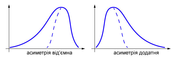
- порівняти середнє, моду, медіану, коефіцієнт асиметрії
- показати довірчій інтервал.
Created with wxMaxima.
The source of this Maxima session can be downloaded here.